Options are a cornerstone of modern financial markets, allowing investors and traders to speculate on price movements, hedge against risk, and optimize their portfolios. But how exactly are these instruments priced? At the heart of options valuation lies a complex interplay of mathematics, market assumptions, and risk factors. The most famous model—Black-Scholes—revolutionized the industry, providing a standardized way to determine fair value. However, real-world markets have shown that no single formula perfectly accounts for all intricacies. In this in-depth guide, we’ll explore how options are priced, delve into the Black-Scholes model, examine its underlying assumptions, discuss alternative models, and provide a comprehensive understanding that goes far beyond the headline formulas.
Table of Contents
1. What Are Options? A Quick Overview

Options are derivative contracts that give the holder the right—but not the obligation—to buy or sell an underlying asset at a predetermined strike price before or at the time of expiration. The two main types of options are:
- Call Options: Provide the right to buy an underlying asset at a specified strike price.
- Put Options: Provide the right to sell an underlying asset at a specified strike price.
The underlying assets can be stocks, indexes, currencies, commodities, or even cryptocurrencies. Options are versatile instruments used for hedging risk, generating income, and speculative trading. But their value at any given moment is not as straightforward as simply comparing the current market price to the strike price—there is a time-sensitive and probabilistic element that makes pricing more complex.
2. Fundamentals of Option Pricing

Option pricing starts from a foundational understanding of value components and the market conditions that ensure fair pricing. Let’s break down the key concepts.
2.1 Intrinsic Value vs. Time Value
- Intrinsic Value: This is the difference between the current underlying price and the option’s strike price, but only if that difference is favorable to the option holder.
- For a call option, intrinsic value = max(Spot Price – Strike Price, 0).
- For a put option, intrinsic value = max(Strike Price – Spot Price, 0).
- Time Value: Even if the option is not currently “in-the-money” (i.e., has no intrinsic value), it may still have value because there is time remaining until expiration. As time passes, there’s a possibility the underlying asset’s price could move favorably, making the option worth more.
The total price of an option (often called its “premium”) is the sum of its intrinsic value and its time value. Early in the life of an option, time value typically represents a significant portion of the premium.
2.2 The No-Arbitrage Principle
A foundational assumption in pricing models is the concept of no-arbitrage. Arbitrage is a risk-free profit made by exploiting price discrepancies between identical or similar instruments. If an option were mispriced, traders could construct strategies that lock in risk-free profits. Such opportunities, however, are quickly eliminated by market participants, driving prices back to fair values. All modern pricing models assume that no-arbitrage conditions must hold, serving as the bedrock of rational pricing.
2.3 Put-Call Parity
Put-Call Parity is a key relationship in European-style options (those that can only be exercised at expiration). It states that the price of a call option, minus the price of a put option with the same strike and expiration, is equal to the current underlying asset price minus the discounted strike price.
Formally:
Call – Put = Spot Price – (Strike Price discounted at the risk-free rate)
This relationship ensures consistency between the prices of calls and puts. If put-call parity didn’t hold, traders could construct arbitrage strategies to earn risk-free profits, which the market would quickly correct.
3. The Black-Scholes Model: A Historic Breakthrough

When Fischer Black, Myron Scholes, and Robert Merton developed their option pricing formula in the early 1970s, it represented a seismic shift in financial theory. Their work transformed options from speculative side bets into rigorously priced financial instruments, enabling explosive growth in the derivatives markets.
3.1 The Origin and Significance
Before Black-Scholes, option pricing was largely guesswork and heuristic. The Black-Scholes model provided an elegant, closed-form solution that quickly gained traction. In 1997, Myron Scholes and Robert Merton were awarded the Nobel Prize in Economic Sciences for the model’s profound impact on finance. (Fischer Black had passed away prior to the award.)
3.2 Key Assumptions
The Black-Scholes model relies on several simplifying assumptions:
- Lognormal Price Distribution: The underlying asset’s price follows a geometric Brownian motion with a constant volatility.
- No Dividends: In the basic form, the model assumes no dividends are paid by the underlying during the option’s life.
- No Arbitrage: Markets are frictionless, and no risk-free arbitrage opportunities exist.
- Constant Risk-Free Rate: The risk-free interest rate remains constant over the option’s life.
- Continuous Trading: You can continuously hedge and rebalance your portfolio with no transaction costs.
3.3 The Black-Scholes Formula Explained
The Black-Scholes formula for a European call option (C) is:
C = S_0 * N(d1) – K * e^{–rT} * N(d2)
Where:
- C = Call option price
- S_0 = Current underlying asset price
- K = Strike price
- r = Risk-free interest rate
- T = Time to maturity (in years)
- N(.) = Cumulative distribution function of the standard normal distribution
- *d1 = [ln(S_0/K) + (r + σ²/2)T] / (σ * sqrt(T))
- d2 = d1 – σ * sqrt(T)
- σ = Volatility of the underlying asset (annualized)
For a put option, a similar formula can be derived using put-call parity. The primary difference lies in adjusting the sign of certain terms.
3.4 Interpreting the Inputs
- Spot Price (S_0): The current market price of the underlying asset.
- Strike Price (K): The predetermined price at which the option holder can exercise the option.
- Volatility (σ): A measure of how much the underlying asset’s returns are expected to fluctuate. Volatility is often the most critical and uncertain input in the formula, as it directly affects the time value of the option.
- Time to Expiration (T): The longer the time until expiration, the greater the potential for price movement, and thus the higher the option value (especially for at-the-money options).
- Risk-Free Rate (r): Typically approximated by the yield on government bonds, the risk-free rate impacts the discounted value of the strike price.
4. The Greeks: Sensitivity Measures in Option Pricing

To manage and understand the risks embedded in an option’s price, traders use metrics known as the Greeks. These measure the sensitivity of an option’s price to various factors.
4.1 Delta
- Definition: Delta measures how much the option’s price changes when the underlying asset’s price moves by one unit.
- Interpretation: A call option with a delta of 0.5 means if the underlying asset’s price rises by $1, the call’s value should increase by approximately $0.50.
4.2 Gamma
- Definition: Gamma measures the rate of change in delta as the underlying price moves. It’s the “second derivative” of the option’s price with respect to the underlying price.
- Interpretation: High gamma suggests delta will change rapidly as the underlying moves, indicating more pronounced curvature in the option’s payoff profile.
4.3 Vega
- Definition: Vega measures the sensitivity of the option’s price to changes in implied volatility.
- Interpretation: A high vega suggests the option’s value is heavily influenced by volatility. Options generally become more valuable as volatility rises because increased volatility implies greater probability of large price movements.
4.4 Theta
- Definition: Theta measures the sensitivity of the option’s price to the passage of time.
- Interpretation: A negative theta means the option loses value as time passes, all else being equal. As expiration approaches, time value erodes, especially if the option is at-the-money.
4.5 Rho
- Definition: Rho measures the sensitivity of the option’s price to changes in the risk-free interest rate.
- Interpretation: A call option with positive rho increases in value as interest rates rise, whereas a put option’s value typically decreases with rising interest rates.
5. Limitations of the Black-Scholes Model

Although the Black-Scholes formula was revolutionary, real markets diverge from its idealized assumptions. Recognizing these limitations is crucial for understanding when and how to adapt the model.
5.1 Unrealistic Assumptions About Volatility
The Black-Scholes model assumes constant volatility. In reality, volatility is dynamic, can spike during market stress, and often exhibits clustering (periods of high volatility followed by more high volatility).
5.2 No Accounting for Dividends in the Original Form
The original Black-Scholes model didn’t incorporate dividend payments. Adjustments are made for dividend-paying stocks by discounting the expected dividend amount from the underlying price or using a continuous dividend yield model.
5.3 The Volatility Smile and Skew
In practice, if you plot implied volatility (the volatility implied by market prices of options) against strike prices, you often get a “smile” or “skew,” not a flat line. This pattern contradicts the model’s assumption of constant volatility and lognormal distributions.
5.4 Non-Lognormal Asset Price Distributions
Empirical evidence shows that asset returns are not perfectly lognormal. Real-world return distributions often have fatter tails and higher peaks than the normal distribution predicts. This leads to discrepancies between theoretical and observed option prices.
6. Alternative and Advanced Pricing Models

As traders and researchers uncovered the limitations of Black-Scholes, new models and approaches emerged to improve accuracy and flexibility.
6.1 The Binomial Model
The Binomial model is a discrete-time model that simulates the evolution of the underlying asset price step-by-step until expiration. At each step, the price can move “up” or “down” by certain factors. By working backward from the terminal payoffs at expiration, the model calculates the option’s fair value at the initial node.
- Advantages: Easy to understand, can incorporate changing volatility or dividends, and flexible for American options.
- Disadvantages: May be computationally intensive for large numbers of time steps and less elegant than Black-Scholes.
6.2 The Trinomial Model
The Trinomial model improves upon the Binomial approach by allowing three possible price moves at each step: up, down, or flat. This additional flexibility can lead to more accurate pricing and can better handle complex payoffs.
- Advantages: More refined than the Binomial model and can approximate continuous models with fewer steps.
- Disadvantages: More computationally involved than the Binomial model.
6.3 Stochastic Volatility Models (e.g., Heston Model)
The Heston model allows volatility itself to be a stochastic (random) variable. Instead of assuming constant volatility, it introduces a separate stochastic process for volatility. This helps capture the observed market phenomena where volatility changes over time and in response to price movements.
- Advantages: More realistic depiction of the underlying price process, can produce volatility smiles and skews naturally.
- Disadvantages: More complex mathematics, often requiring numerical methods for solutions.
6.4 Jump-Diffusion Models
Jump-diffusion models incorporate sudden, large movements (jumps) in the asset price. These jumps could represent significant market events, news releases, or macroeconomic shocks. By combining continuous diffusion (as in Black-Scholes) with discrete jumps, these models can better fit fat-tailed distributions observed in real markets.
- Advantages: Better captures extreme events and market shocks.
- Disadvantages: More complicated calibration and more complex to implement.
6.5 Local Volatility and SABR Models
Local volatility models assume that volatility is a deterministic function of the underlying asset price and time. The Dupire local volatility framework, for example, extracts local volatilities from market prices of options. Similarly, the SABR model (Stochastic Alpha, Beta, Rho) is designed to fit the volatility smile across strikes and maturities.
- Advantages: Provides a more direct fit to the observed market structure of option prices.
- Disadvantages: Requires complex calibration and may not always perfectly capture market dynamics.
7. Practical Considerations for Traders and Investors
In the real world, option pricing models are not just academic tools; they are embedded in trading strategies, portfolio management, and risk management systems.
7.1 How Market Makers Use Models
Market makers rely on pricing models to set bid and ask quotes for options. They adjust their prices and hedge positions dynamically, using tools like the Black-Scholes model and advanced variants to ensure that they remain neutral to market movements. Their trading desks monitor deltas, gammas, vegas, and other Greeks to maintain balanced portfolios.
7.2 Implied Volatility and Market Expectations
Instead of using historical volatility directly, many traders back-solve the Black-Scholes model with the option’s current market price to find the “implied volatility.” Implied volatility is a forward-looking metric that reflects the market’s expectation of future volatility. Changes in implied volatility often say more about market sentiment and fear than underlying asset price movements alone.
- Example: A sudden increase in implied volatility for S&P 500 Index options might indicate that traders anticipate turbulent times ahead, possibly due to upcoming economic announcements or geopolitical tensions.
7.3 Calibration of Models in Practice
In practice, traders and quantitative analysts must calibrate their chosen models to current market data. Calibration involves adjusting parameters (like volatility surfaces, jump intensities, or correlation structures) to best fit observed option prices. This ensures that the theoretical model aligns closely with the actual trading environment.
- Example: A volatility surface shows implied volatilities for various strikes and maturities. A trading desk might use local volatility or SABR models to fit this surface as accurately as possible, then use the calibrated model for pricing exotic options.
7.4 Technology and Algorithmic Approaches
The computational challenges of advanced models have led to the development of numerical techniques and advanced algorithms. Monte Carlo simulations, finite difference methods, and Fourier transform techniques are routinely employed, assisted by high-speed computing environments. As technology evolves, machine learning and neural networks are increasingly explored for pricing complex derivatives and discovering patterns in volatility surfaces.
8. Real-World Examples and Illustrations
Understanding theory is one thing; seeing how it’s applied makes the concepts more tangible.
8.1 Simple Pricing with the Binomial Model
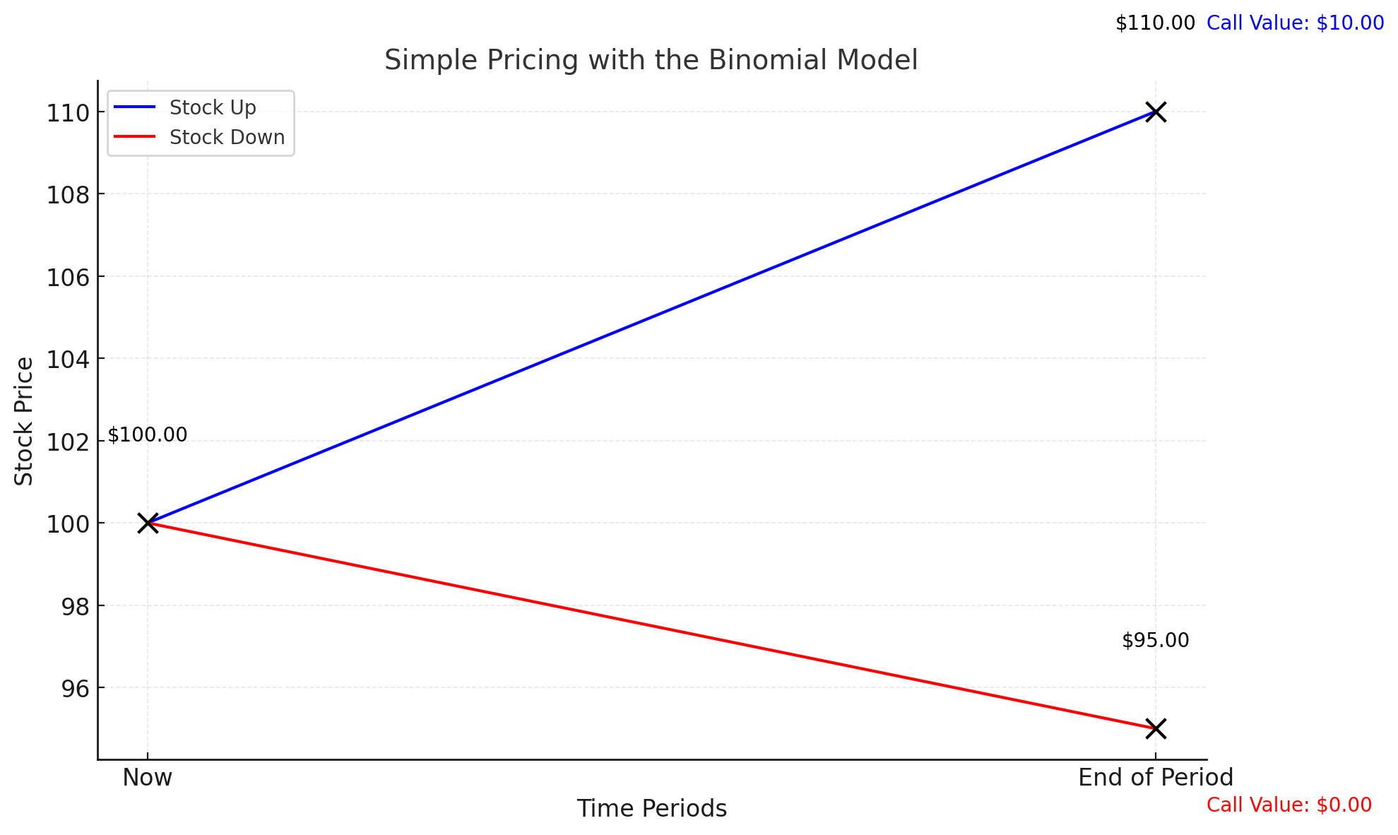
Example: Consider a one-period binomial model for a stock currently trading at $100. Suppose that after one period (one month), the stock can either go up by 10% (to $110) or down by 5% (to $95). If we’re valuing a call option with a strike of $100 that expires in one month, we start by computing the option’s value at the end of the period:
- If the stock ends up at $110: The call’s intrinsic value is $110 – $100 = $10.
- If the stock ends down at $95: The call is worthless (0 intrinsic value).
We then discount these payoffs back to the present using the risk-free rate and the “risk-neutral probabilities” derived from no-arbitrage conditions. Let’s say the risk-neutral probability is p. The present value (option price) would be:
*Call Price = e^{–rT} * [p * (10) + (1–p)0].
By calibrating p and plugging in the risk-free rate, we get a fair value for the call. This simple exercise lays the foundation for the more complex continuous-time models like Black-Scholes.
8.2 Understanding Volatility Smiles in Equity Markets
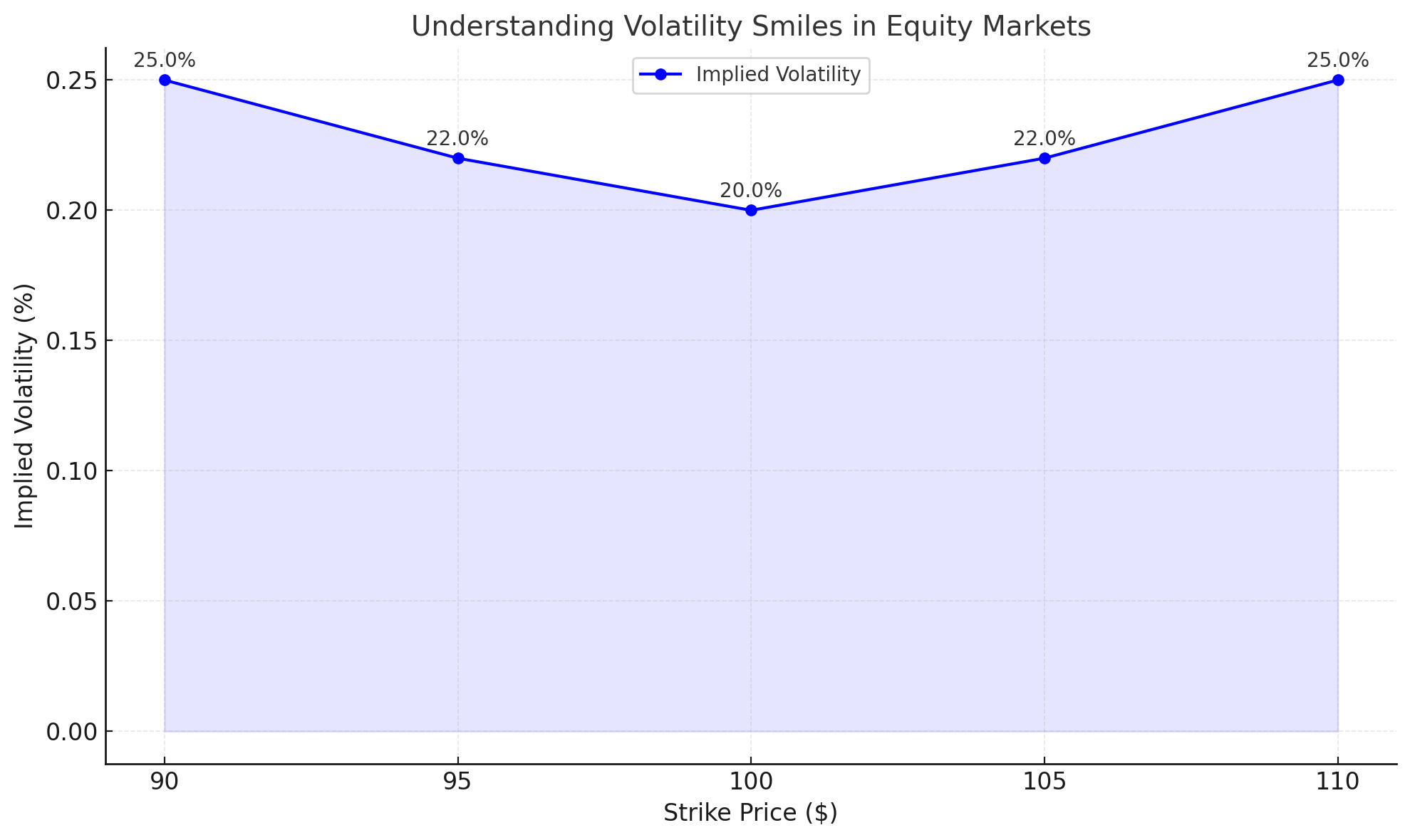
Imagine you’re looking at options on a popular stock. The at-the-money options might have an implied volatility of 20%. However, deep out-of-the-money puts might have an implied volatility of 25%, while deep out-of-the-money calls might have 22%. Plotting implied volatility versus strike price would reveal a skew: the market is pricing greater volatility (and thus probability of extreme moves) for far out-of-the-money strikes.
This “smile” or “skew” can arise from the market’s anticipation of rare events or asymmetry in the probability distribution of future stock prices. Understanding this helps traders select models that better capture market psychology and avoid underpricing tail risks.
9. Conclusion and Future Developments
The question of how options are priced begins with the now-classic Black-Scholes model, but it doesn’t end there. While Black-Scholes gave the financial world a powerful starting point, real markets have proven more complex and nuanced. Traders and analysts must consider time-varying volatility, jumps, liquidity constraints, and many other factors that influence option values.
In today’s markets, advanced pricing frameworks—stochastic volatility, jump-diffusion, local volatility models, and even machine learning approaches—are employed to capture the subtleties of price formation. As markets evolve, and as technology expands our computational capabilities, the pursuit of ever-more-accurate pricing methodologies continues.
Yet one principle remains consistent: the goal of option pricing models is to reflect reality as closely as possible while maintaining mathematical tractability. By staying informed about model limitations, evolving approaches, and practical calibration techniques, traders and investors can better navigate the complexities of the options market and make more informed decisions.
In Summary:
- Black-Scholes laid the groundwork for modern option pricing.
- The Greeks help measure risks and sensitivities.
- Real markets exhibit features like volatility skew and jumps that the classic model doesn’t fully capture.
- Alternative models and advanced techniques address these complexities, providing more realistic valuations.
- Ongoing research and technological innovation continue to refine how options are priced, ensuring that markets remain efficient, transparent, and accessible to a broad range of participants.
By understanding the theory, mastering the tools, and recognizing the limitations and advanced methods available, market participants can confidently approach the world of options pricing—Black-Scholes and beyond.
